Back to the Oscillation Lessons
Download FAQ Document for Lesson and Simulations
- Project Overview
- General characteristics of complex systems
- Project goals
- Lessons and simulations
- Iceberg visual
- Simulation Use
- Levels and intended audiences
- Setting up the simulation
- Menus, buttons and links
- Home
- Slidebars
- Knobs
- Buttons
- Graphs
- Lesson Use
- Printing
- Level of guidance
- Making predictions
- Assessment information
- About the Visual Tools
- Behavior-over-time graphs
- Causal loops
- Stock/flow maps
- Background documents
- Troubleshooting
- The simulation gives me a timeout message.
- The text and the graphics are all “mixed up.”
- The simulation behavior doesn’t make sense.
- I can’t see the entire line on the graph.
a. General characteristics of complex systems
"The intuitively obvious ‘solutions’ to social problems are apt to fall into one
of several traps set by the character of complex systems."
—Jay W. Forrester, World Dynamics
What are the characteristics of complex systems referred to by Dr. Forrester?
- Cause and effect are not closely related in time or space.
- Action is often ineffective due to application of low-leverage policies (treating the symptoms, not the problem).
- High-leverage policies are difficult to apply correctly.
- The cause of the problem is within the system.
- Collapsing goals results in a downward spiral.
- Conflicts arise between short-term and long-term goals.
- Burdens are shifted to the intervener.
Top of Document
b. Project goals
Led by a partnership between MIT Professor Emeritus Jay W. Forrester and the Creative Learning Exchange, the goal of the project is to create online curricula for ages five and above that will illustrate the characteristics of complex systems. In exploring the nature of complex social systems, the curricula address questions such as – why do such systems resist policy changes? Why are short-term and long-term responses to corrective action often at odds with each other? How can leverage points be applied to bring about desirable change in social systems?
The goals of the project are grounded in the belief that an abstract level of understanding of social systems will help prepare future citizens to actively shape their society.
Top of Document
c. Lessons and simulations
The lessons and simulations are based upon the fourth characteristic of complex systems, the cause of the problem is within the system.
Five interdisciplinary areas are covered in this series of lessons, utilizing a family of models that all generate oscillation. Oscillation in real-world systems is often considered problematic rather than a consequence of system structure. This progression of lessons helps students understand that undesirable behavior can be a consequence of system structure and not a result of outside, uncontrollable influences. In other words, a system that oscillates does so because it has an inherent tendency to do so. See the next page for a visual representation of the project components. You can click on any part of the diagram for additional information.
Top of Document
d. Iceberg Visual
Click on the image below to see the iceberg in a larger size.

Top of Document
a. Levels and intended audiences
The main topics for the simulations in this series are:
-
Spring Dynamics
- Interpersonal Relationships
- Population Dynamics
- Logistic Growth
- Predator/Prey Interactions
- Predator/Prey/Biomass Interactions
- Burnout
- Economics of Commodities
Most simulations in the series have three possible levels of use – Level A (ages 5+), Level B (ages 9+), and Level C (ages 13+). Note that these age recommendations are in no way absolute, but generally speaking, the Level A simulations are intended for younger students, while the Level C simulations are intended for older students. That said, it is also possible to use multiple levels of a simulation for differentiation purposes. Students who need material at a higher or lower reading level could use a different version of the simulation along with its accompanying handouts.
Top of Document
b. Setting up the simulation
Menus, buttons and links
- Each simulation level has a standardized menu system. Levels A and B simulations have button menu systems; Level C simulations have a hyperlink system.
Level A Menu:

Level B Menu:

Level C Menu Example:
Home

- Every screen has a “Home” button available. This button returns the user to the front title screen of the simulation.
Slidebars
- Types
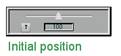
- Slidebars are one method for manipulating the settings for a simulation. Some of the slidebars are based on a general range, with no values showing. Here’s one example within the Level A – Spring simulation.

- Other simulations have slidebars that include numerical settings. The lesson might call for the student to set a slidebar to a particular number.
- Setting a slidebar
- Setting a slidebar is as simple as moving the little rectangular lever to the right or left to select higher or lower settings.
- Slidebars that have visible numerical values can also be set by clicking on the value in the middle and typing in the desired number.
- Slidebars must be set according the indicated minimum and maximum values. For example, if a range is 0 - 2000, the user will not be able to type in a value that exceeds 2000.
- Slidebars must be set by certain increments, depending on the variable. For example, if a range is 0 - 2000, then the increments may go up or down by increments of 100.
Knobs

- General
- Most of the Level C simulations contain one or more knobs on the control panel screen. These are manipulated in a fashion similar to slidebars, with minimum and maximum values.
- Setting a knob
- A knob is set by moving the black dot around to the desired setting.
Buttons
- Buttons are used throughout a simulation for different purposes, including navigation among the pages of the simulation, initiating a new simulation run, and resetting the simulation graphs. Depending on the level of the simulation, these buttons may be rectangular images or resemble links on a webpage.
Graphs
- General
- Graphs show the simulation results as a behavior-over-time graph. Graphs are also covered in the next section on visual tools.

- The simulation lesson handouts for the B and C levels (but not the A levels) presume that students know how to create, title, label, and create a key for a line graph.
- Options
- Some graphs may have multiple pages. To see the additional graphs, click on the tab
 at the bottom, left of the graph pad. Each time you click, the next graph appears. After clicking through all the graphs, you’ll return again to the first one.
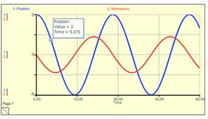
- To see the actual values at any point on a graph line, click and hold the mouse arrow right on the line at the point you’d like to check. A box will appear showing the value at a particular point in time.
Top of Document
Lesson Use
a. Printing
Unless indicated otherwise, handouts are formatted for double-sided printing. Some handouts are optional, depending on prior student experience. For example, one lesson includes an optional handout based on having read a particular book.
b. Level of guidance
The lessons, particularly for Level C, are designed so students can work as independently as possible while moving through the simulations. For other levels, especially Level A simulations, students may need instruction to guide them through the procedures of setting up and running the simulation. Depending on student ages, reading levels, and ability to be self-directed, you may choose to eliminate some of the more guided handouts. Creating an environment in which students can explore the simulation in an organic fashion is an option. Consideration should then be given to developing alternate methods to have students demonstrate understanding of the embedded concepts.
c. Making predictions and comparing results
Key elements embedded within handouts include having students make predictions prior to viewing results, and then comparing those predictions to actual graphical data. These tasks, in addition to being strongly connected to multiple curricular standards, are key to enhancing the ability of students to think deeply about what is causing particular results.
d. Assessment information
Although example student responses to some handout questions are included in lesson plans, no official answer keys are provided. Most questions are written to allow for multiple “correct” answers. Some questions are seeking an opinion or an interpretation, along with evidence. These questions by their very nature do not lend themselves to the creation of a discrete set of answers.
Top of Document
About the Visual Tools
a. Behavior-over-time graphs
 The variable being measured is always on the y-axis of the graph. Time is displayed on the x-axis. Depending on the context, the time frame could be short (measured in seconds) or long (measured in years). Most of the models in this series produce a variety of oscillatory behaviors, although other trends are also possible. See the simulation background documents for additional information about typical behavior patterns.
Top of Document
b. Causal loops
A causal (or feedback) loop diagram is another visual tool that shows the structure of a system. A feedback loop tells a story about how a system operates. Any given system may have multiple interconnected loops. Arrows between any two elements indicate a cause-and-effect relationship: If the first element rises, then it causes the second element either to rise or fall. Depending on the relationship, different symbols are used. See the loop below along with the key explaining the different symbols.

Top of Document
c. Stock/flow maps
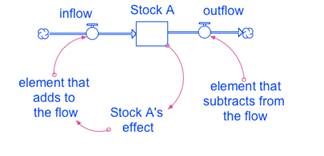
 A stock/flow map represents the structure of the system. The parts of the map along with the underlying mathematical assumptions define the nature of the interdependent relationships among the parts. This structure is based on assumptions about how the system (whether it be a spring or relationships on the playground) really works.
In its simplest form, a stock represents an accumulated amount and the flow (or flows) represent the rate at which the stock goes up or down. Other elements impact one or more flows, either adding to or subtracting from a stock.
Top of Document
d. Background documents
Each simulation has an accompanying background document. These documents give the teacher more detail on the model structure and its resulting behaviors, including limitations of the model and ideas for discussion.
Top of Document
Troubleshooting
a. “The simulation gives me a timeout message.”
When running the simulation online, you may occasionally experience a “time out” message. This can occur for a variety of reasons, but the most common is when nothing on the simulation screen has been clicked for a while. If this happens, simply reload the page and return to the screen you last visited.
Top of Document
b. “The text and the graphics are all ‘mixed up.’”
Occasionally, the development team updates simulations to improve them. If your computer browser has an old version saved in its memory, this can cause the simulation to display erroneous information. To fix this issue, you need to clear the cache from your browser. Browsers (e.g. Internet Explorer, Firefox, Safari) have different procedures for doing this, so see the help documentation for your browser if needed.
Top of Document
c. “The simulation behavior doesn’t make sense.”
Each of the simulation models in this series has limitations and is valid only when used within those limitations. If settings that exceed the model parameters are put into the simulation, the user may experience behavior on the graph that doesn’t make sense.
For example, the animal population simulation shows the population trends for the animals included on the handouts. If the user tries to input data for an animal that has a very long lifespan and that frequently has many offspring, an exponential growth pattern may be produced. In reality, something else would limit the population growth, but the parameters of the simulation are not able to handle that extreme scenario.
See the accompanying background documents for additional information about the limitations of each model.
Top of Document
d. “I can’t see the entire line on the graph.”
In some cases, you may input settings that cause the behavior to go beyond the scale of a particular graph. If this occurs, most of the simulations have a button that allows the user to see the full graph. Note that no scale is set for this special graph, but rather a new scale (on the y-axis) is created with each new run.
Top of Document